


Ok, back to “musical mapping” temporarily. As I’ve said I’m proposing a talk for this fall’s Annual Meeting of the North American Cartographic Information Society on the relationships between musical and geographical space and ways of “mapping” those relationships, applied specifically to The Last Island. Again these ideas tend toward the academic, and the mapping part is still a work-in-progress, so my main goal in showcasing them here is to pace myself and test them out; I’m mostly curious as to how well the imagery communicates the broad points even without all the explanation. Maybe parts of it are interesting purely as artwork? (Probably not yet.) If the whole thing is too abstract, then just listen to the piece if you haven’t yet—I’ve heard enough reactions that I can promise you’ll find it soothing :-) .
For a quick recap of the mapping approach (much more detail here if you dare), I’m analyzing the piece in terms of three categories of elements: environmental, visual (painted), and musical. The three categories correspond/align with each other to varying degrees, i.e. the music evokes the painted imagery (the slides in the video) which in turn depicts natural environments/landscapes along the island journey. Since I wrote the piece before selecting the visual imagery, setting up the framework for this mapping process, or knowing that I was going to do either one of those things at all, those correspondences vary in their strength and clarity. Even if the composition had come at the end instead of the beginning that might still be the case, given that slavishly tying the choice and progression of musical elements to, say, rainfall or elevation might not have produced the most listenable piece; that would've been a bad outcome despite my OCD compulsion to treat it like a research subject. (I’m realizing that it fits in well though with my cartography-not-painting framing of the worldviews.)The point of the mapping exercise then is two-fold: 1) to figure out the best ways of visually representing those correspondences, so that they can be absorbed more quickly and clearly than in the 12-minute duration of the piece, and 2) to get a visual sense of how strong those correspondences actually turned out to be, given what I just said about not obsessing too much about them during the composition process.
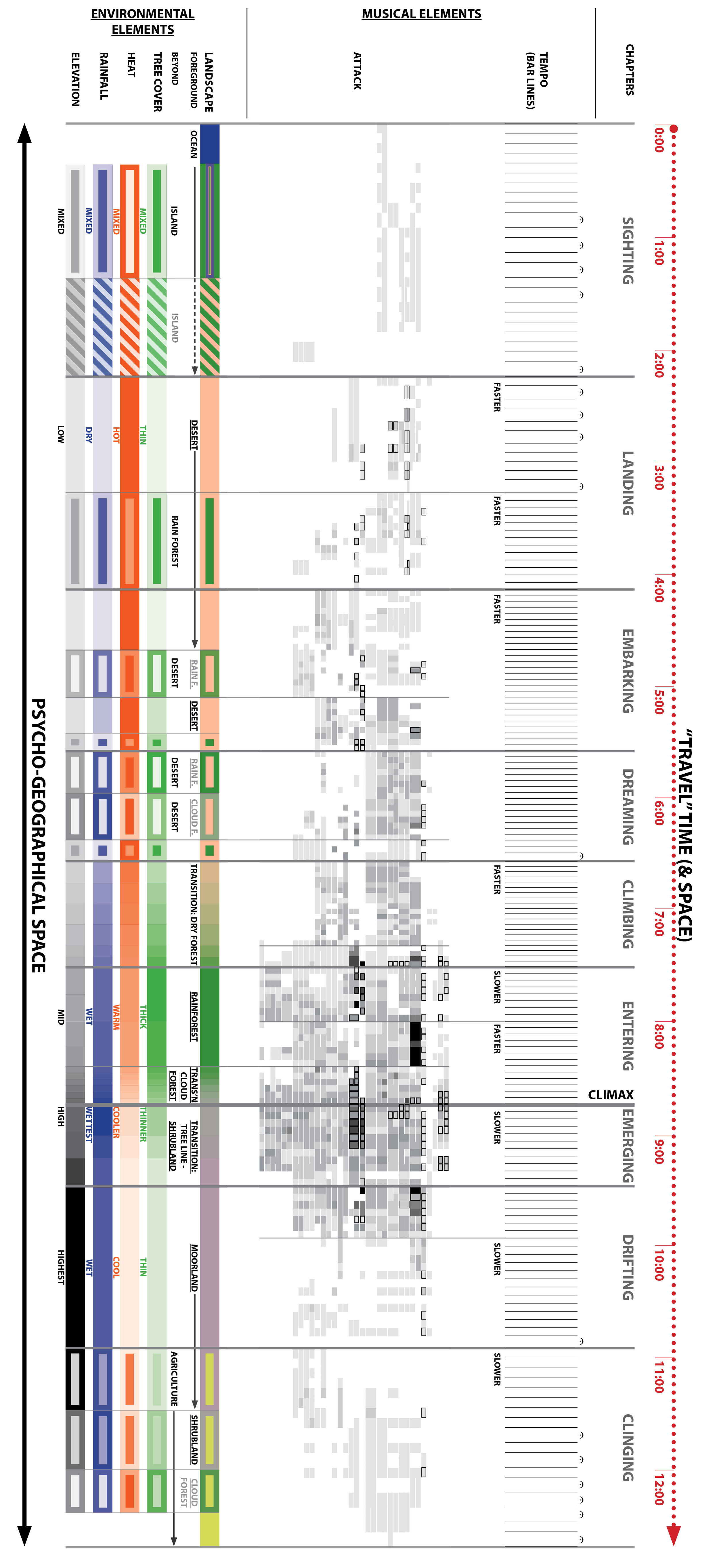
Turning to the maps/diagrams themselves, again think of the bands representing the environmental elements as abstractions, layered on top of one another, of the island landscape seen from above (and seen from within in the painted slides). Think of the musical elements as abstractions of the printed musical score, standing on edge as it winds through the visual/physical landscape. And given the length of the diagrams I’ve oriented the image vertically; I’ll be referring to top, bottom, left and right as if you were looking at the sheet horizontally. (Go to the website to see slightly larger versions.)
Musical Elements: Note Length
The maps I shared before illustrated the “structural elements” of theme and path—in quotes because they’re not musical “elements” themselves so much as frameworks for organizing what I consider the actual elements of pitch, tempo, dynamics, instrumentation, etc…Here I’ll go into two of these actual musical elements, attack and tempo, grouped together because they’re both aspects of note length. (“Rhythm” is too, but since I’m more concerned with general variations in note length from measure to measure or section to section than from note to note, I don’t plan to deal with it.)
Attack. I still need a better term for this—I mean it as the number of discrete notes, whether of the same pitch or different pitches (“note” implies pitch, so that term won’t work) begun or “attacked” within some given time interval such as a measure. (A note tied over from the previous measure doesn’t count.) I’ve tallied the number of attacks per measure for each voice/instrument (each voice/instrument represented by a horizontal band), and depicted the count on a grayscale gradient from light (1-2 attacks per measure) to dark (27-32 per measure, unscientifically increasing the range at the upper end assuming that adding a note is less perceptible when there are more of them).
The outlines of varying thicknesses around some of the boxes represent effects (occurring somewhere in that measure) where it’s impossible to count the number of attacks or where the notes are played so quickly that it’s hard to evaluate how important they are—think of these as another layer of activity on top of the tally of “regular” notes. From thinnest to thickest outline, again representing a gradient from least to most activity, these are 1) grace notes, 2) rolled chords or glissandi (mostly on the harp), and 3) trills (including rolls on percussion).
(Incidentally I’ve arranged voices/instruments differently than in a standard score, ordering percussion, strings, winds, and brass from top to bottom. With this arrangement the map gets “thicker” where the percussion and brass are the most active, rather than just denser (with internal gaps getting filled in). Thickening seems a bit more impactful at a glance than densifying, plus the typical score arrangement is completely arbitrary for what I’m trying to communicate.)
Tempo. Number of attacks per measure only captures ones aspect of note length, because measures don’t all take up the same amount of time even if the time signature (number of beats) is constant. So, the relative tempo speeds need to be illustrated as a separate map or layer. There’s an easy way to do that: since I’ve set up the diagrams for time to progress at a constant rate from left to right (see the ticker tape at the top of the sheet), bar lines (measure divisions) will be farther apart at slow tempos than at fast tempos, and if they contain fermatas (holds) at any tempo. Analogous to the attack diagram, this results in a darker/denser appearance (i.e. more activity) where the tempo is faster.
As with the theme and path diagrams, the vertical lines are my attempt to call out the alignments and misalignments between the different types of elements; basically they represent the edges between experiential zones. This time I’ve added a higher level of zone, separated by the thicker lines, labeled at the top of the sheet as “chapters.” Think of these as broader divisions of the musical narrative based on activity or mood; in the video the labels appear on the first slide of each chapter.
Ideally the attack and tempo diagrams would be superimposed to create a more complete picture of note length at glance. I’ve tried this (see the sheet below), but the bar line density fades into the background unless I thicken the lines so much as to be distracting. I’ve also tried subdividing the measures with additional lines to further darken/densify the fast tempos, but that just makes everything look darker. Another option, which would take a lot of work but I might do it anyways, is to merge the note tally and beats-per-minute components of each measure into a single number—so for example a measure with 8 attacks but a tempo twice as fast as some chosen baseline tempo would functionally have 16. This would create a more concise and accurate illustration of note length, but also more opaque. (For any of you who can visualize this before I re-calculate a few thousand measures—thoughts?)
Despite all this complexity, I’m hoping what’s clear is a broad-brush correspondence between “high intensity” zones across environmental and musical elements. The zone where elevation, temperature, rainfall, and tree cover are cumulatively greatest/highest—most saturated in terms of color—roughly lines up with the shortest note durations in terms of attack and tempo and what I consider to be the “climax” of narrative at the beginning of the “Emerging” chapter, namely emerging from the cloud forest into the high, bright moorland zone. (This makes me think I might add “sunlight” as an environmental element?)
There is one somewhat obvious misalignment here—the fastest tempos (densest bar lines) actually occur well before the climax point. The chapter label “Climbing” provides a clue though, and later maps will illustrate it better: this could be considered the most “energetic” part of the piece in terms of physical exertion and mental anticipation.
Slow and Fast, Long and Short
Part of me is questioning my decision to represent time linearly from left to right, so that slow tempo zones get stretched out in space and fast zones get compressed. It seemed the most logical way to go at the time. But shouldn’t slower speeds, loosely representing slower walking speeds and less coverage of space, look more compressed and therefore static on the musical map? And consistent with what I said earlier about the map looking “thicker” in zones of greater intensity, shouldn’t a faster traversing of space appear wider on the page, so that overall the map looks “bigger”? I’ve gone ahead and tested out this other option, which I’ve labeled “distorted time” (again, note the ticker tape) and placed side-by-side with the original “constant time” version on the sheet below. In both cases I’ve overlaid the tempo map (the bar lines) with the attack map as I suggested above.
I’ve also added the visual element (the row of slides from the video) back in to show that the time distortion also has the effect of (slightly) un-distorting space: the slides are a little more equal in size relative to the constant-time version. Overlaying the musical score/”journey” on a traditional physical map without any perceptible spatial distortion, as opposed to one of my worldviews where certain landscape fragments can be enlarged to imply more time spent there, would be possible with the distorted-time version because it’s the score that would be instead compressed or stretched out.

I haven’t decided yet which version is the better visual representation of relative travel speed and, combined with the light-to-dark attack gradient, overall intensity of experience. Any thoughts on which map shows the middle section of the score as more “active” than the beginning and end?
Going with the distorted-time version might mean that the tempo diagram disappears and gets incorporated into the attack diagram in the way I described above—multiplying the attack tally by some factor representing relative tempo. Otherwise the two diagrams, whether superimposed or not, contradict each other: shorter note lengths mean darker in terms of attacks but lighter (more widely-spaced bar lines) in terms of tempo.
Alright, more musical maps to come later—probably with a little less theory involved!
Darren